Data Operation
name <- c("Alex", "Rosie", "Greg")
gender <- c("M", "W", "M")
age <- c(18,19,20)
a_score <- c(98, 99, 100)
b_score <- c(1, 2, 3)
df <- data.frame(name, gender, age, a_score, b_score)
创建新变量
transform(df, ...): 对df进行...操作
df <- transform(df, age = age + 1, avg_score = (a_score+b_score)/2)
   name gender age a_score b_score avg_score
1  Alex      M  19      98       1      49.5
2 Rosie      W  20      99       2      50.5
3  Greg      M  21     100       3      51.5
变量重编码
# 未指定区间
grades <- c("D", "C", "B", "A")
tmp <- quantile(stu_tot, probs=c(0.4, 0.6, 0.8))
break_pts <- c(-Inf, tmp, Inf)
score_level <- cut(scores, break_pts, labels=grades, ordered_result=TRUE)

# 指定区间
scores <- c(50, 70, 93, 67)
grades <- c("F", "D", "C", "B", "A")
break_pts <- c(-Inf, 60, 70, 80, 90, Inf)
score_level <- cut(scores, break_pts, labels=grades, ordered_result=TRUE)
注意
cut(x, breaks, labels = NULL,
    include.lowest = FALSE, right = TRUE, dig.lab = 3,
    ordered_result = FALSE, …)

right=T 表示左开右闭
right=F 表示左闭右开
补充
pretty(x, …)
# S3 method for default
pretty(x, n = 5, min.n = n %/% 3,  shrink.sml = 0.75,
       high.u.bias = 1.5, u5.bias = .5 + 1.5*high.u.bias,
       eps.correct = 0, …)

n
integer giving the desired number of intervals. Non-integer values are rounded down.

min.n
nonnegative integer giving the minimal number of intervals. If min.n == 0, pretty(.) may return a single value.

pretty(1:15)                    # 0  2  4  6  8 10 12 14 16
pretty(1:15, high.u.bias = 2)   # 0  5 10 15
pretty(1:15, n = 4)             # 0  5 10 15
pretty(1:15 * 2)                # 0  5 10 15 20 25 30
pretty(1:20)                    # 0  5 10 15 20
pretty(1:20, n = 2)             # 0 10 20
pretty(1:20, n = 10)            # 0  2  4 ... 20
变量的重命名
# 法一
fix(df) # 跳出来一个编辑框

# 法二
names(df)[1] <- "sname"

# 法三
install.packages("plyr")
library(plyr)
df <- rename(df, c(name="sname", age="sage"))
缺失值
df == NA永远不会为T,因为NA不可比- R不会把
Inf或NaN标记为NA
is.na(c(1,2,3))
## [1] FALSE FALSE FALSE
is.na(df)
      name gender   age a_score b_score
[1,] FALSE  FALSE FALSE   FALSE   FALSE
[2,] FALSE  FALSE FALSE   FALSE   FALSE
[3,] FALSE  FALSE FALSE   FALSE   FALSE

df$test <- NA
df
##    name gender age a_score b_score test
## 1  Alex      M  18      98       1   NA
## 2 Rosie      W  19      99       2   NA
## 3  Greg      M  20     100       3   NA
df[is.na(df)]
## [1] NA NA NA
df[is.na(df)] <- T
df
##    name gender age a_score b_score test
## 1  Alex      M  18      98       1 TRUE
## 2 Rosie      W  19      99       2 TRUE
## 3  Greg      M  20     100       3 TRUE
日期

# 获得当前日期
Sys.Date()
## [1] "2021-10-24"
date()
## [1] "Sun Oct 24 20:34:34 2021"

# 字符串转换为日期
as.Date(c("1970-1-5", "2017-9-12"))
as.Date("1/5/1970", format="%m/%d/%Y")
# 默认format=yyyy-mm-dd

# 指定输出形式
format(Sys.Date(), format="%B %d %Y")
## [1] "十月 24 2021"

# 算术运算
sdate <- as.Date("2021-02-13")
edate <- as.Date("2022-02-13")
days <- edate - sdate
days
## Time difference of 365 days
# 或
difftime(edate, sdate, units="weeks")
## Time difference of 52.14286 weeks

# 逻辑运算
sdate > edate
## [1] FALSE

# 日期转换为字符串
sdate <- as.character(Sys.Date())
sdate
## [1] "2021-10-24"
类型转换
is.numeric() as.numeric()
排序
一些绘图需要排序预处理,如打乱的时序数据
# order() 默认是升序,加一个减号变为降序
new_df <- df[order(df$a_score, -df$b_score),]
# 优先按a_score升序,若a_score相同则按b_score降序
合并
1. 添加列

id1 <- c(2, 3, 4, 5, 7)
heights <- c(62, 65, 71, 71, 67)
df1 <- data.frame(id = id1, heights)

id2 <- c(1, 2, 6:10)
weights <- c(147, 113, 168, 135, 142, 159, 160)
df2 <- data.frame(id = id2, weights)

df1
##   id heights
## 1  2      62
## 2  3      65
## 3  4      71
## 4  5      71
## 5  7      67

df2
##   id weights
## 1  1     147
## 2  2     113
## 3  6     168
## 4  7     135
## 5  8     142
## 6  9     159
## 7 10     160

merge(df1, df2, all = FALSE) # colnames(df1) ∩ colnames(df2) = id
##   id heights weights
## 1  2      62     113
## 2  7      67     135

merge(df2, df1, all = FALSE)
##   id weights heights
## 1  2     113      62
## 2  7     135      67

merge(df1, df2, by = "id", all = TRUE)
##    id heights weights
## 1   1      NA     147
## 2   2      62     113
## 3   3      65      NA
## 4   4      71      NA
## 5   5      71      NA
## 6   6      NA     168
## 7   7      67     135
## 8   8      NA     142
## 9   9      NA     159
## 10 10      NA     160

merge(df1, df2, by = "id", all.x = TRUE)
##   id heights weights
## 1  2      62     113
## 2  3      65      NA
## 3  4      71      NA
## 4  5      71      NA
## 5  7      67     135

merge(df1, df2, by = "id", all.y = TRUE)
##   id heights weights
## 1  1      NA     147
## 2  2      62     113
## 3  6      NA     168
## 4  7      67     135
## 5  8      NA     142
## 6  9      NA     159
## 7 10      NA     160
# 按行名进行合并
z <- matrix(c(0,0,1,1,0,0,1,1,0,0,0,0,1,0,1,1,0,1,1,1,1,0,0,0,"RND1","WDR", "PLAC8","TYBSA","GRA","TAF"), nrow=6, dimnames=list(c("ILMN_1651838","ILMN_1652371","ILMN_1652464","ILMN_1652952","ILMN_1653026","ILMN_1653103"),c("A","B","C","D","symbol")))

t<-matrix(c("GO:0002009", 8, 342, 1, 0.07, 0.679, 0, 0, 1, 0,
        "GO:0030334", 6, 343, 1, 0.07, 0.065, 0, 0, 1, 0,
        "GO:0015674", 7, 350, 1, 0.07, 0.065, 1, 0, 0, 0), nrow=10, dimnames= list(c("GO.ID","LEVEL","Annotated","Significant","Expected","resultFisher","ILMN_1652464","ILMN_1651838","ILMN_1711311","ILMN_1653026")))

> z
             A   B   C   D   symbol
ILMN_1651838 "0" "1" "1" "1" "RND1"
ILMN_1652371 "0" "1" "0" "1" "WDR"
ILMN_1652464 "1" "0" "1" "1" "PLAC8"
ILMN_1652952 "1" "0" "1" "0" "TYBSA"
ILMN_1653026 "0" "0" "0" "0" "GRA"
ILMN_1653103 "0" "0" "1" "0" "TAF"

> t
             [,1]         [,2]         [,3]
GO.ID        "GO:0002009" "GO:0030334" "GO:0015674"
LEVEL        "8"          "6"          "7"
Annotated    "342"        "343"        "350"
Significant  "1"          "1"          "1"
Expected     "0.07"       "0.07"       "0.07"
resultFisher "0.679"      "0.065"      "0.065"
ILMN_1652464 "0"          "0"          "1"
ILMN_1651838 "0"          "0"          "0"
ILMN_1711311 "1"          "1"          "0"
ILMN_1653026 "0"          "0"          "0"

cbind(t, z[, "symbol"][match(rownames(t), rownames(z))])
             [,1]         [,2]         [,3]         [,4]
GO.ID        "GO:0002009" "GO:0030334" "GO:0015674" NA
LEVEL        "8"          "6"          "7"          NA
Annotated    "342"        "343"        "350"        NA
Significant  "1"          "1"          "1"          NA
Expected     "0.07"       "0.07"       "0.07"       NA
resultFisher "0.679"      "0.065"      "0.065"      NA
ILMN_1652464 "0"          "0"          "1"          "PLAC8"
ILMN_1651838 "0"          "0"          "0"          "RND1"
ILMN_1711311 "1"          "1"          "0"          NA
ILMN_1653026 "0"          "0"          "0"          "GRA"
df1 <- data.frame(name, age, gender)
df2 <- data.frame(name, a_score, b_score)
df  <- merge(df1, df2, by="name")
   name age gender a_score b_score
1  Alex  18      M      98       1
2  Greg  20      M     100       3
3 Rosie  19      W      99       2
# dff <- merge(df1, df2, by=c("name", "age")) 也有这样的语法

# 直接合并,不指定索引
df <- cbind(df1, df2)
   name age gender  name a_score b_score
1  Alex  18      M  Alex      98       1
2 Rosie  19      W Rosie      99       2
3  Greg  20      M  Greg     100       3
2. 添加行
两个df必须拥有相同的变量。不过顺序不必相同
df1 <- data.frame(name, age, gender)
df2 <- data.frame(name, age, gender)
df  <- rbind(df1, df2)
子集操作
访问见 Grammar
丢弃变量
# 丢弃name与gender列
# 法一
tmp <- names(df) %in% c("name", "gender")
new_df <- df[!tmp]

# 法二
df$name <- df$gender <- NULL
随机抽样
# 从第一行到最后一行中,随机抽2个,无放回
mysample <- df[sample(1:nrow(df), 2, replace=F), ]
SQL语句
install.packages('sqldf')
library(sqldf)
new_df <- sqldf('select * from df where name=\'Alex\'', row.names=T) # 保留行名
常用函数
1. 数学函数P86 统计函数P88
2. scale()
- 归一化 默认均值为0 方差为1
- 存在非数值列会报错
new_df <- scale(df)
# 若要化为均值为M,方差为SD
new_df <- scale(df) * SD + M
# 若想要只针对某个列(col_name)进行标准化
new_df <- transform(df, col_name=scale(col_name)*SD+M)
3. 概率函数
set.seed(1234) # 指定种子,用于复现,但只是一次性的,每次随机都要重新指定
runif(5) # 生成5个服从均匀分布U(0,1)的伪随机数
runif(5, min=0, max=100) # U[0, 100]
rnorm(10) # 生成标准正态分布的随机数
rnorm(10,mean=1,sd=4) # 生成...随机数 sd是标准差
mvrnorm(100, mu=mean, Sigma=sigma) # 生成100个服从N(mean, sigma)
# mean是平均值向量,sigma是协方差矩阵

dnorm(0) # 表示标准正态分布密度 就是咱们记得表达式,像凸字形
## [1] 0.3989423
pnorm(0) # 标准正态分布函数 形似 sigmoid
## [1] 0.5
sample(x, size, replace = FALSE, prob = NULL):从 x 中选 size 个
- size: 个数
- replace: 若为T,则有放回的抽
4. 字符处理函数P93
5. 其他实用函数
option(digits=2) # 后续都保留两位小数

x <- 1:10
length(x)
## [1] 10
m <- matrix(1:20, nrow=4)
length(m)
## [1] 20
df <- data.frame(name=c("A", "B", "C"), score=1:3)
length(df)
## [1] 2
arr <- array(1:20, dim=c(2,2,5))
length(arr)
## [1] 20

cut(x, 5) # 分割为一个有着5个水平的因子
##  [1] (0.991,2.8] (0.991,2.8] (2.8,4.6]   (2.8,4.6]   (4.6,6.4]
## [6] (4.6,6.4]   (6.4,8.2]   (6.4,8.2]   (8.2,10]    (8.2,10]
## 5 Levels: (0.991,2.8] (2.8,4.6] (4.6,6.4] ... (8.2,10]
cut(x, breaks=0:3)
##  [1] (0,1] (1,2] (2,3] <NA>  <NA>  <NA>  <NA>  <NA>  <NA>  <NA>
## Levels: (0,1] (1,2] (2,3]

labels = c("差", "中", "优")
cut(x, breaks=0:3, labels)
##  [1] 差   中   优   <NA> <NA> <NA> <NA> <NA> <NA> <NA>
## Levels: 差 中 优

cut(x, breaks=0:3, labels, ordered_result=TRUE)
##  [1] 差   中   优   <NA> <NA> <NA> <NA> <NA> <NA> <NA>
## Levels: 差 < 中 < 优

pretty(x, 5) # 创建美观的分割点
## [1]  0  2  4  6  8 10

quantile(x, c(.8, .6, .4, .2)) # 返回一根向量
## 80% 60% 40% 20%
## 8.2 6.4 4.6 2.8

x <- list(1:2, 'aaa', matrix(1:20,nrow=4))
"["(x, 2) # 返回x的第二个元素,仍是列表
## [[1]]
## [1] "aaa"

cat("我后面会有一个空格", "我前面有一个空格", "不会自动\n换行")
## 我后面会有一个空格 我前面有一个空格 不会自动
## 换行

cat(..., file='xxx', append=FALSE)
6. 批量操作函数
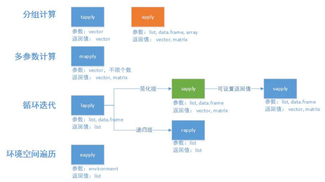
apply(x, MARGIN, FUN)
输入一个df或matrix,输出vector或list或array
MARGIN=1表示行,MARGIN=2表示列
若MARGIN=1,则表示对x的每一行进行FUN操作
即 MARGIN 为多少,就保留这些维度,即若 MARGIN = c(1, 2),那么最后的 shape 是 (len(第一维度), len(第二维度))
apply(X,       # Array, matrix or data frame
      MARGIN,  # 1: columns, 2: rows, c(1, 2): rows and columns
      FUN,     # Function to be applied
      ...)     # Additional arguments to FUN
m <- matrix(1:20, nrow=4)
apply(m, 1, mean) # 对每一行求平均值
apply(m, 1, mean, trim=0.2) # 对每一行的20%~80%的部分求平均

x <- array(1:24, c(3,4,2))
apply(x, c(1, 2), sum) # 在第三维度值求和
     [,1] [,2] [,3] [,4]
[1,]   14   20   26   32
[2,]   16   22   28   34
[3,]   18   24   30   36

# Example
# 给出有2列的矩阵,求斜边长
apply(m, 1, function(x) sqrt(sum(x^2)))
sapply(x, FUN, options)
返回一个长度与 X 一致的向量(通过length()函数可以反向推出处理的单元),每个元素为 FUN 计算出的结果,且分别对应到X中的每个元素。
sapply(X,   # Vector, list or expression object
       FUN, # Function to be applied
       ..., # Additional arguments to be passed to FUN
       simplify = TRUE,  # If FALSE returns a list. If "array" returns an array if possible
       USE.NAMES = TRUE) # If TRUE and if X is a character vector, uses the names of X
# 输入列表
l <- list(a=1:10, b=matrix(1:20, nrow=4))
sapply(l, sum)
##  a   b
## 55 210

# 输入向量
movies <- c("SPYDERMAN","BATMAN","VERTIGO","CHINATOWN")
movies_lower <-sapply(movies, tolower)
movies_lower
##   SPYDERMAN      BATMAN     VERTIGO   CHINATOWN
## "spyderman"    "batman"   "vertigo" "chinatown"
tolower(movies)
## [1] "spyderman" "batman"    "vertigo"   "chinatown"

# 输入df
df
##   age score
## 1  18    99
## 2  19    98
## 3  20    97
sapply(df, sum)
## age score
##  57   294

# 输入矩阵
m <- matrix(1:20, nrow=4)
sapply(m, sum)
## [1]  1  2  3  4  5  6  7  8  9 10 11 12 13 14 15 16 17 18 19 20
# 事与愿违是因为
length(m)
## [1] 20
sum(m)
## [1] 210
mean(m)
## [1] 10.5

# FUN使用参数
sapply(x, "[", 2) # 若x是一个列表,则取列表中每一个元素的第2个元素 见课本P99

# 可以基于这个实现向量切片
below_ave <- function(x) {
    ave <- mean(x)
    return(x[x > ave])
}
dt_s <- sapply(df, below_ave)
##   age score
##  20.0  51.5
dt_l <- lapply(df, below_ave)
## $age
## [1] 20

## $score
## [1] 51.5

identical(dt_s, dt_l)
## [1] TRUE

# 实例,假设df$name 由Alex Sean类似格式组成,现要求从中抽取出姓和名
name <- strsplit((df$name), " ")
fname <- sapply(name, "[", 2)
lname <- sapply(name, "[", 1)
lapply(x, FUN, options)
返回一个长度与 X 一致的列表,每个元素为 FUN 计算出的结果,且分别对应到X中的每个元素。
与apply()区别在于输出的是list,且无需MARGIN
lapply(X,   # List or vector
       FUN, # Function to be applied
       ...) # Additional arguments to be passed to FUN
# 输入列表
l <- list(a=1:10, b=matrix(1:20, nrow=4))
lapply(l, sum)
## $a
## [1] 55

## $b
## [1] 210

# 输入向量
movies <- c("SPYDERMAN","BATMAN","VERTIGO","CHINATOWN")
movies_lower <-lapply(movies, tolower)
movies_lower
## [[1]]
## [1] "spyderman"

## [[2]]
## [1] "batman"

## [[3]]
## [1] "vertigo"

## [[4]]
## [1] "chinatown"

unlist(movies_lower)
## [1] "spyderman" "batman"    "vertigo"   "chinatown"

# 输入df
df
##   age score
## 1  18    99
## 2  19    98
## 3  20    97
lapply(df, sum)
## $age
## [1] 57

## $score
## [1] 294

# 输入矩阵
m <- matrix(1:20, nrow=4)
lapply(m, sum)
## [[1]]
## [1] 1

## [[2]]
## [1] 2
## ...
# 事与愿违是因为
length(m)
## [1] 20
tapply(X, INDEX, FUN): 对一维数据按 label 分组后分别 apply fun
tapply(X,                # Object you can split (matrix, data frame, ...)
       INDEX,            # List of factors of the same length
       FUN,              # Function to be applied to factors (or NULL)
       ...,              # Additional arguments to be passed to FUN
       default = NA,     # If simplify = TRUE, is the array initialization value
       simplify = TRUE)  # If set to FALSE returns a list object
set.seed(2)

data_set <- data.frame(price = round(rnorm(25, sd = 10, mean = 30)),
                       type = sample(1:4, size = 25, replace = TRUE),
                       store = sample(paste("Store", 1:4),
                                      size = 25, replace = TRUE))

head(data_set)
  price type   store
1    21    2 Store 2
2    32    3 Store 3
3    46    4 Store 4
4    19    3 Store 4
5    29    1 Store 4
6    31    3 Store 4

price <- data_set$price
store <- data_set$store
type <- factor(data_set$type,
               labels = c("toy", "food", "electronics", "drinks"))
# Mean price by product type
mean_prices <- tapply(price, type, mean)

mean_prices
        toy        food electronics      drinks
   39.50000    30.33333    32.20000    29.33333
class(mean_prices)
## "array"

# 等价于
by(data_set, data_set$type, function(x) mean(x$price))
data_set$type: 1
[1] 39.5
------------------------------------------
data_set$type: 2
[1] 30.33333
------------------------------------------
data_set$type: 3
[1] 32.2
------------------------------------------
data_set$type: 4
[1] 29.33333

# 由于array不能用 $ 操作,所以可考虑返回list
# Mean price by product type
mean_prices_list <- tapply(price, type, mean, simplify = FALSE)
mean_prices_list
$toy
[1] 39.5

$food
[1] 30.33333

$electronics
[1] 32.2

$drinks
[1] 29.33333

# Mean price by product type and store
tapply(price, list(type, store), mean)
            Store 1  Store 2 Store 3  Store 4
toy              46 31.00000      49 36.66667
food             26 30.33333      39       NA
electronics      50 29.00000      32 25.00000
drinks           22 40.00000      20 36.00000

# Mean price by product type and store, changing default argument
tapply(price, list(type, store), mean, default = 0)
            Store 1  Store 2 Store 3  Store 4
toy              46 31.00000      49 36.66667
food             26 30.33333      39  0.00000
electronics      50 29.00000      32 25.00000
drinks           22 40.00000      20 36.00000
mapply()
mapply(FUN, …, MoreArgs = NULL, SIMPLIFY = TRUE,
       USE.NAMES = TRUE)
mapply(function(x,y){x^y},x=c(2,3),y=c(3,4))
## [1]  8 81

# the values in y are recycled.
# i.e. for both the values in x the same value (4) of y is used.
mapply(function(x,y){x^y},x=c(2,3),y=c(4))
## [1] 16 81
mapply(function(x,y){x^y},c(a=2,b=3),c(A=3,B=4))
## a  b
## 8 81
mapply(function(x,y){x^y},c(a=2,b=3),c(A=3,B=4),USE.NAMES=FALSE)
## [1]  8 81
# 指定fun中的额外参数
mapply(function(x,y,z,k){(x+k)^(y+z)},c(a=2,b=3),c(A=3,B=4),MoreArgs=list(1,2))
##   a    b
## 256 3125
vapply()
vapply(.x, .f, fun_value, ..., use_names = TRUE)
The vapply function is very similar compared to the sapply function, but when using vapply you need to specify the output type explicitly.
test <- list(a = c(1, 3, 5), b = c(2,4,6), c = c(9,8,7), d=c("A", "B", "C"))

sapply(test, max)
  a   b   c   d
"5" "6" "9" "C"

vapply(test, max, numeric(1))
## Error in vapply(test, max, numeric(1)) : values must be type 'double',
##  but FUN(X[[4]]) result is type 'character'
rapply()
rapply stands for recursive apply, and as the name suggests it is used to apply a function to all elements of a list recursively.
x <- list(1,2,3,4)
rapply(x,function(x){x^2},class=c("numeric"))
## [1]  1  4  9 16

x <- list(1,2,3,4,"a")
rapply(x,function(x){x^2},class=c("numeric"))
## [1]  1  4  9 16
7. 聚合函数
aggregate(x, by, FUN)
FUN只能是单返回值函数
整合数据,相当于group by by_list and apply fun on each group
by中的变量必须在一个list中,即使只有一个元素;可以在列表中自定义各组的别名
# Data frame
aggregate(x,               # R object
          by,              # List of variables (grouping elements)
          FUN,             # Function to be applied for summary statistics
          ...,             # Additional arguments to be passed to FUN
          simplify = TRUE, # Whether to simplify results as much as possible or not
          drop = TRUE)     # Whether to drop unused combinations of grouping values or not.

# Formula
aggregate(formula,             # Input formula
          data,                # List or data frame where the variables are stored
          FUN,                 # Function to be applied for summary statistics
          ...,                 # Additional arguments to be passed to FUN
          subset,              # Observations to be used (optional)
          na.action = na.omit) # How to deal with NA values
aggregate(mtcars, by=list(mtcars$cyl, mtcars$gear), FUN=mean, na.rm=TRUE)
# group by(cyl, gear) and apply mean on each group
aggregate(mtcars$disp, by=list(mtcars$cyl, mtcars$gear), FUN=mean, na.rm=TRUE)
  Group.1 Group.2        x
1       4       3 120.1000
2       6       3 241.5000
3       8       3 357.6167
4       4       4 102.6250
5       6       4 163.8000
6       4       5 107.7000
7       6       5 145.0000
8       8       5 326.0000
# 等价于
aggregate(disp~cyl+gear, data=mtcars, FUN=mean, na.rm=TRUE)
  cyl gear     disp
1   4    3 120.1000
2   6    3 241.5000
3   8    3 357.6167
4   4    4 102.6250
5   6    4 163.8000
6   4    5 107.7000
7   6    5 145.0000
8   8    5 326.0000

# 统计频率
aggregate(chickwts$feed, by = list(chickwts$feed), FUN = length)
aggregate(feed ~ feed, data = chickwts, FUN = length) # Equivalent

states <- data.frame(state.region, state.x77)
##                 state.region Population Income Illiteracy Life.Exp Murder HS.Grad Frost   Area
## Alabama                South       3615   3624        2.1    69.05   15.1    41.3    20  50708
## Alaska                  West        365   6315        1.5    69.31   11.3    66.7   152 566432
## Arizona                 West       2212   4530        1.8    70.55    7.8    58.1    15 113417
aggregate(states$Illiteracy, by=list(state.region), FUN=mean)
#        Group.1        x
1     Northeast 1.000000
2         South 1.737500
3 North Central 0.700000
4          West 1.023077
by(data, INDICES, FUN)
indices是一个因子或因子组成的列表(定义分组),fun是任意函数
即将data按照indices因子水平进行分组,然后对每组应用fun函数
df
##    name gender age a_score b_score
## 1  Alex      M  18      98       1
## 2 Rosie      W  19      99       2
## 3  Greg      M  20     100       3
by(df, df$gender, function(x) mean(x[,4]))
## df$gender: M
## [1] 99
## ------------------------------------------------
## df$gender: W
## [1] 99
table()
类似count on group-by
默认会忽略NA,需要NA的话,添加参数useNa='ifany'
table(Arthritis$Improved) # 统计频数

##  None   Some Marked
##    42     14     28

table(Arthritis$Improved, Arthritis$Treatment)
##         Placebo Treated
##  None        29      13
##  Some         7       7
##  Marked       7      21
8. 转置t()
df <- data.frame(name, gender, age, a_score, b_score)
row.names(df) <- df$name # 或rownames(df) <- df$name
df$name <- NULL
t(df)
        Alex  Rosie Greg
gender  "M"   "W"   "M"
age     "18"  "19"  "20"
a_score " 98" " 99" "100"
b_score "1"   "2"   "3"